RLHF: Reward Models + PPO#

This is the “everything included” era of the chapter’s deletion narrative: a learned reward model, a critic, a reference model, and a full PPO loop — four networks in memory at once. RLHF is the pipeline that turned base models into assistants (Christiano et al. 2017 for the idea; Stiennon et al. 2020 for summarization; Ouyang et al. 2022 — InstructGPT — for the recipe everyone copied). Everything the later pages delete, they delete from here, so this page sets up each component carefully enough that its removal will mean something.

The pipeline#

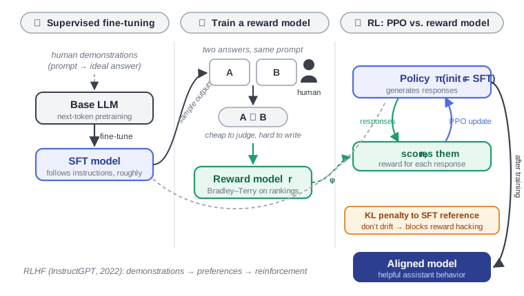
Three stages:

1. Supervised fine-tuning (SFT). Fine-tune the base model on human-written demonstrations. This produces $\pi_{\text{ref}}$ — a competent policy and, just as importantly, the anchor everything downstream is regularized toward.
2. Reward model training. Sample pairs of responses from the SFT model, have humans pick the better one, and fit a scalar reward model $r_\phi$ to the rankings.
3. RL fine-tuning. Optimize the policy against $r_\phi$ with PPO, tethered to $\pi_{\text{ref}}$ by a KL penalty.

Why a reward model at all? Because RL needs millions of reward queries and humans are slow and expensive — but also for a subtler reason visible in the figure: responses are cheap to judge, hard to write. Ranking two answers takes seconds; writing a demonstration takes minutes. Preferences are the cheaper signal, and the reward model is the machine that converts a finite pile of them into an unlimited supply of reward queries.

Stage 1: supervised fine-tuning is behavioral cloning#

The first stage looks like ordinary supervised learning, but it has an exact RL name. Given demonstrations $\mathcal{D}_{\text{SFT}} = \{(x, y^*)\}$ of prompts paired with human-written responses, SFT does maximum likelihood, which by the factorization of Section 4.1 is token-level cross-entropy over the response:

In RL terms this is behavioral cloning: imitate an expert policy’s actions in the expert’s own states, with no reward anywhere. Two consequences of that reading are worth stating precisely.

MLE is a forward KL. Writing $p^*(\cdot \mid x)$ for the demonstrators’ conditional distribution, the population SFT loss decomposes as

so up to the constant entropy term, SFT minimizes the forward KL — the mass-covering direction: $\pi_\theta$ is punished wherever demonstrators put mass that it doesn’t. Note the pleasing symmetry with Stage 3, which regularizes with the reverse KL — the mode-seeking direction. The pipeline first spreads the policy over everything humans do, then sharpens it toward what they prefer; the two stages literally optimize the two directions of the same divergence.

Cloning inherits cloning’s limits. The loss evaluates $\pi_\theta$ only in expert states — prefixes $y^*_{\lt t}$ written by humans. At generation time the model conditions on its own prefixes, and small errors compound: one off-distribution token leads to a state no demonstration covered, where nothing constrains the next token (the classic compounding-error argument for behavioral cloning; Ross et al. 2011). And imitation is bounded by the demonstrator — MLE has no mechanism for exceeding the quality of $\mathcal{D}_{\text{SFT}}$. Both limits are exactly what Stages 2–3 exist to lift: preferences supply a signal between model samples rather than at human samples, and RL evaluates the policy on its own states.

In code, the loss is the Section 4.1 primitive with one extra detail — the mask excludes prompt tokens, not just padding, so no gradient flows through predicting the prompt:

def sft_loss(logits, input_ids, response_mask):
    """
    logits:        (B, T, V) model outputs on the full sequence [prompt; response]
    input_ids:     (B, T)    the same sequence, as targets
    response_mask: (B, T)    1 on response tokens, 0 on prompt tokens and padding
    """
    logps = torch.log_softmax(logits[:, :-1], dim=-1)             # predict token t+1 from prefix t
    target_logps = logps.gather(-1, input_ids[:, 1:].unsqueeze(-1)).squeeze(-1)
    mask = response_mask[:, 1:]                                    # align with shifted targets
    return -(target_logps * mask).sum() / mask.sum()               # mean NLL over response tokens

The output of this stage, $\pi_{\text{ref}}$, then plays two roles at once: initialization for the policy and the frozen anchor of the KL leash.

Note what this loss does not involve: sampling. SFT is teacher forcing — at every position the model conditions on the human-written prefix $y^*_{\lt t}$, never on its own generations, and the whole response is trained in one parallel forward pass. The model that enters this stage is the full pretrained network; SFT is the same next-token objective continued on a dataset roughly six orders of magnitude smaller, with the loss masked to response tokens. Generation appears in the pipeline for the first time in Stage 2, when response pairs are sampled for humans to rank.

Stage 2: from preferences to a reward#

The standard preference model is Bradley–Terry: given responses $y_w$ (chosen) and $y_l$ (rejected) to prompt $x$, assume

where $\sigma$ is the logistic function. Maximum likelihood on a preference dataset $\mathcal{D} = \{(x, y_w, y_l)\}$ gives the reward-model loss

Two observations worth pausing on:

• This is just logistic regression on reward differences — pairwise classification with the reward gap as the logit. No RL has happened yet.
• The reward is identified only up to a per-prompt constant. Adding any $c(x)$ to $r_\phi$ leaves every difference — and hence the loss — unchanged. This shift-invariance is not a bug: policy-gradient methods are themselves invariant to prompt-dependent baselines (the zero-mean advantage trick from Section 3), so the unidentified constant is exactly the part that never mattered. File this away — it is one of the two facts DPO exploits on the next page.

Architecturally, the reward model is the SFT model with its language-model head swapped for a scalar head, read out at the final token:

import torch
import torch.nn as nn
import torch.nn.functional as F

class RewardModel(nn.Module):
    """A language-model backbone with a scalar head on the last token."""
    def __init__(self, backbone, hidden_size):
        super().__init__()
        self.backbone = backbone
        self.v_head = nn.Linear(hidden_size, 1, bias=False)

    def forward(self, input_ids, attention_mask):
        h = self.backbone(input_ids, attention_mask)      # (B, T, H) last hidden states
        last = attention_mask.sum(-1).long() - 1          # index of final real token
        h_last = h[torch.arange(h.size(0)), last]         # (B, H)
        return self.v_head(h_last).squeeze(-1)            # (B,) scalar rewards

def reward_model_loss(r_chosen, r_rejected):
    """Bradley-Terry negative log-likelihood on preference pairs."""
    return -F.logsigmoid(r_chosen - r_rejected).mean()

Stage 3: the KL-regularized objective#

Optimizing $r_\phi$ unconstrained would be a mistake, because $r_\phi$ is a proxy fit on a finite dataset — and unconstrained optimization against a proxy invites reward hacking (Goodhart’s law, an old friend to every experimentalist). The objective that RLHF actually optimizes is

with $\beta$ trading reward against drift from the SFT anchor. This objective has a closed-form solution — the Gibbs variational principle from the mathematics companion, at last on stage:

where $Z(x)$ is the (intractable) per-prompt normalizer. The optimum is the reference policy, exponentially tilted toward reward. We cannot sample from $\pi^*$ — computing $Z(x)$ means summing over all possible responses — which is why Stage 3 exists: PPO is how we approximate the tilt. But the formula itself is the second fact DPO will exploit: it can be solved for $r_\phi$ in terms of $\pi^*$. Hold that thought until Section 4.3.

Reading the KL two ways. The penalty is simultaneously a statistical device (do not trust the reward model outside the distribution it was trained on) and an optimization device (keep the policy near a region where language remains fluent). The dashed tether in the pipeline figure is carrying both loads.

In practice: PPO over tokens#

The objective above is stated at the sequence level, but the implementation lives in the token-level MDP of Section 4.1 — this is exactly the regime where the two views diverge, because everything below acts per-token.

Per-token reward shaping. The KL penalty is not applied as one sequence-level number; it is distributed along the trajectory as a dense per-token reward, with the reward model’s score added at the final token:

This turns the sparse terminal reward into a partially dense signal — the one shaping term the LLM setting gives us for free:

def shaped_rewards(token_logps, ref_logps, mask, terminal_reward, beta):
    """
    token_logps, ref_logps, mask: (B, T)   terminal_reward: (B,)
    Returns per-token rewards (B, T): -beta * KL estimate at every step,
    plus the reward-model score added at each sequence's final token.
    """
    rewards = -beta * (token_logps - ref_logps) * mask     # dense KL penalty
    last = mask.sum(-1).long() - 1                          # final token index
    rewards[torch.arange(rewards.size(0)), last] += terminal_reward
    return rewards

The PPO update. From here it is Section 3 verbatim: a critic $V_\psi(s_t)$ over partial sequences, GAE on the shaped rewards $\tilde{r}_t$ (with $\gamma = 1$, per the finite-horizon setting of 4.1), and the clipped surrogate applied at every token:

def ppo_loss(token_logps, old_logps, advantages, mask, eps=0.2):
    """
    token_logps: (B, T) under the current policy (requires grad)
    old_logps:   (B, T) under the policy that generated the batch (no grad)
    advantages:  (B, T) e.g. from GAE over the shaped rewards
    """
    ratio = torch.exp(token_logps - old_logps)
    unclipped = ratio * advantages
    clipped = torch.clamp(ratio, 1 - eps, 1 + eps) * advantages
    per_token = -torch.minimum(unclipped, clipped)
    return (per_token * mask).sum() / mask.sum()

Note the two different old policies hiding in this code: old_logps belongs to $\pi_{\theta_{\text{old}}}$, the policy that generated the batch (it moves every iteration), while ref_logps in the shaping function belongs to $\pi_{\text{ref}}$, the SFT model (frozen forever). Conflating them is the single most common confusion about RLHF — the first deep dive below takes it apart.

The bill#

Count what Stage 3 keeps in memory: the policy (training), the reference (frozen, for the KL), the reward model (frozen, for scoring), and the critic (training, for GAE) — four transformer-scale networks, two of them updating, plus PPO’s hyperparameter surface ($\beta$, $\epsilon$, GAE-$\lambda$, minibatch schedule) and its famous implementation sensitivity (Engstrom et al. 2020). It works — every major assistant through ~2023 was built this way — but the cost begs a question the closed-form solution above already whispered:

if we can write down the optimal policy, do we need the RL loop at all?

That is Section 4.3: Direct Preference Optimization.

References.

• Christiano et al. (2017), Deep RL from Human Preferences;
• Stiennon et al. (2020), Learning to Summarize from Human Feedback;
• Ouyang et al. (2022), Training Language Models to Follow Instructions (InstructGPT);
• Gao, Schulman & Hilton (2023), Scaling Laws for Reward Model Overoptimization;
• Engstrom et al. (2020), Implementation Matters in Deep Policy Gradients;
• Schulman (2020), Approximating KL Divergence (blog note).
• Ross et al. (2011), A Reduction of Imitation Learning and Structured Prediction to No-Regret Online Learning (DAgger)