The Mathematics of Policy Gradient Methods#

Companion page to Policy-Based Deep RL: that page supplies intuition; this one supplies statements and proofs. Notation is self-contained. Throughout, expectations are assumed to exist and differentiation-under-the-integral is assumed valid (dominated convergence; in particular the support of $\pi_\theta$ must not depend on $\theta$).

1. Setup and notation#

An MDP $(\mathcal{S}, \mathcal{A}, P, R, \gamma)$ with $\gamma \in [0,1)$; a parameterized stochastic policy $\pi_\theta(a \mid s)$, differentiable in $\theta$. A trajectory $\tau = (s_0, a_0, s_1, a_1, \dots)$ has density

return $G(\tau) = \sum_{t \ge 0} \gamma^t r_t$ with $r_t = R(s_t, a_t)$, and return-to-go $G_t = \sum_{k \ge 0} \gamma^k r_{t+k}$.

The objective and the standard value functions:

and the advantage

Define the (unnormalized) discounted state-visitation measure

The expectations can be rewritten for $\mathbb{E}_{\tau \sim p_\theta}[\cdot] = \mathbb{E}_{s\sim\rho^{\pi_\theta}, a\sim\pi_\theta}[\cdot]$.

2. The policy gradient theorem#

Theorem 1 (trajectory form).

Proof. Exchange gradient and integral, apply the identity $\nabla_\theta p_\theta = p_\theta \nabla_\theta \log p_\theta$ (chain rule), and expand the log of the trajectory density:

Now $\log p_\theta(\tau) = \log \rho_0(s_0) + \sum_t \log \pi_\theta(a_t|s_t) + \sum_t \log P(s_{t+1}|s_t,a_t)$, and only the middle sum depends on $\theta$ — the initial distribution and dynamics differentiate to zero. $\square$

The vanishing of the dynamics terms is the substantive content: the estimator requires no model and never differentiates the reward.

Corollary 2 (causality / reward-to-go).

Proof. Expand $G(\tau) \sum_t \nabla \log \pi_t$ and consider a cross-term $\gamma^k r_k \nabla_\theta \log \pi_\theta(a_t|s_t)$ with $k < t$ (a past reward multiplying a future score). Condition on the history up to $s_t$; the inner expectation contains the factor $\mathbb{E}\big[\nabla_\theta \log \pi_\theta(a_t|s_t) \mid s_t\big] = \nabla_\theta \int \pi_\theta(a|s_t)\, da = \nabla_\theta 1 = 0$. All such terms vanish, leaving each score paired only with rewards from its own time onward.

The corresponding math derivation is as follows:

Since

we have

$\square$

Remark (the missing $\gamma^t$ in practice). Implementations — and the intuitive statement on the main page — drop the $\gamma^t$ prefactor, weighting every timestep’s score equally while still discounting inside $G_t$ (or $\hat A_t$). This estimator is not the gradient of the discounted objective: it corresponds to the undiscounted state-visitation measure, and in general is not the gradient of any fixed objective (Thomas, 2014; Nota & Thomas, 2020). It is used anyway because the exact $\gamma^t$ weighting starves late timesteps of learning signal. This is a genuine, rarely-advertised gap between the theorem and the code.

Lemma 3 (baselines are free). For any function $b : \mathcal{S} \to \mathbb{R}$,

so replacing $G_t$ by $G_t - b(s_t)$ in Corollary 2 leaves the gradient unbiased.

Proof. Same score-function identity as above, conditioned on $s_t$: $b(s_t)$ is measurable given $s_t$, and the conditional mean of the score is zero. $\square$

Remark (variance). The variance-minimizing baseline is

which is a score-weighted value and approximated by the unweighted $V^\pi(s)$ in practice. With that choice the weight becomes the advantage, and we obtain the state-visitation form of the theorem (Sutton et al., 2000):

3. Advantage estimation and GAE#

$A^\pi$ is unknown and must be estimated from data; every practical algorithm is a choice of estimator $\hat A_t$. Two extremes, given a learned value function $V_\phi \approx V^\pi$: the Monte-Carlo estimate $\hat A_t = G_t - V_\phi(s_t)$ (unbiased given $V_\phi = V^\pi$, high variance), and the one-step TD estimate

(low variance, biased whenever $V_\phi \ne V^\pi$). Note $\mathbb{E}[\delta_t \mid s_t, a_t] = A^\pi(s_t,a_t)$ when $V_\phi = V^\pi$: the TD error is itself an advantage estimator.

Generalized advantage estimation (GAE) (Schulman et al., 2016) interpolates by exponentially weighting multi-step estimators. Define the $k$-step advantage

Then

where the second and third equality follow by exchanging the two sums and summing the geometric series in $\lambda$, respectively. The knob recovers both extremes: $\lambda = 0$ gives $\delta_t$; $\lambda = 1$ telescopes to $G_t - V_\phi(s_t)$. Bias decreases and variance increases monotonically in $\lambda$.

4. Off-policy evaluation of a new policy: the surrogate objective#

Trust-region methods rest on an exact identity.

Lemma 4 (performance difference; Kakade & Langford, 2002). For any two policies $\pi', \pi$:

where the two right-hand sides are equal by definition of the unnormalized visitation measure $\rho^{\pi'}$ from §1 — the time-sum is absorbed into the measure. ($\rho^{\pi'}$ has total mass $1/(1-\gamma)$; papers using the normalized measure state the lemma with a $\tfrac{1}{1-\gamma}$ prefactor instead.)

Proof. By the Bellman equation for $\pi$, the advantage is a conditional expectation over the next state only:

Substitute along a trajectory of $\pi'$ (tower property: the outer expectation over $\tau \sim \pi'$ absorbs the inner one, since $s_{t+1}$ in the trajectory is distributed as $P(\cdot \mid s_t, a_t)$):

The second sum telescopes exactly — consecutive terms cancel, leaving only the boundary: $\gamma^{T} V^{\pi}(s_{T}) - V^{\pi}(s_0)$. Now let $T \to \infty$: with bounded rewards, $\lvert V^\pi \rvert \le R_{\max}/(1-\gamma)$, so $\gamma^T V^{\pi}(s_T) \to 0$, and the first sum converges to $J(\pi')$. Hence the left side equals $J(\pi') - \mathbb{E}_{s_0 \sim \rho_0}[V^{\pi}(s_0)] = J(\pi') - J(\pi)$. $\square$

The lemma is exact but impractical: the expectation is under $\rho^{\pi'}$, the state distribution of the policy we have not yet deployed. The surrogate replaces it with the old distribution and importance-weights the actions:

$L_\pi$ matches $J(\pi') - J(\pi)$ to first order at $\pi' = \pi$ (same value, same gradient).

The error is controlled by how far the state distributions $\rho^{\pi}$ drift:

Theorem 5 (monotonic improvement bound; TRPO form). With $\epsilon = \max_s \mathbb{E}_{a\sim\pi'} \lvert A^\pi(s,a) \rvert$ and $\alpha = \max_s D_{\mathrm{TV}}(\pi'(\cdot|s), \pi(\cdot|s))$,

Maximizing the right-hand side each iteration guarantees $J$ never decreases. Since $D_{\mathrm{TV}}^2 \le \tfrac{1}{2} D_{\mathrm{KL}}$ (Pinsker), the penalty can be stated in KL, and TRPO’s practical algorithm solves $\max_{\pi'} L_\pi(\pi')$ subject to $\bar D_{\mathrm{KL}}(\pi, \pi') \le \delta$.

5. PPO: the clipped surrogate#

Proximal policy optimization (PPO, Schulman et al., 2017) replaces the constraint by a pointwise modification of the integrand. With $\rho_t(\theta) = \pi_\theta(a_t|s_t) / \pi_{\theta_{\mathrm{old}}}(a_t|s_t)$:

Three properties substitute for a proof of Theorem-5-style guarantees (PPO has none):

1. First-order agreement: at $\theta = \theta_{\mathrm{old}}$, $\rho_t = 1$, the clip is inactive, and $\nabla L^{\mathrm{CLIP}} = \nabla L_\pi$, i.e., PPO ascends the true surrogate initially.
2. One-sided pessimism: the outer $\min$ makes $L^{\mathrm{CLIP}}$ a pointwise lower bound on the unclipped surrogate; clipping only ever removes incentive, never adds it.
3. Zero marginal incentive past the trust region: if $\hat A_t > 0$ and $\rho_t > 1+\epsilon$ (or $\hat A_t < 0$ and $\rho_t < 1-\epsilon$), the gradient of that term is exactly zero — the sample stops arguing for further movement. Note the asymmetry: clipping caps the reward for moving, but a sample can still push the ratio back into the region.

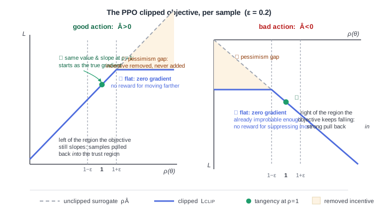
Even these are properties of the objective, not of the learning dynamics: in practice, multiple epochs on a batch can carry ratios well outside the clip range (the clipped sample’s gradient is zero, but other samples keep moving the shared parameters), and much of PPO’s empirical edge traces to code-level choices — advantage normalization, learning-rate annealing, value clipping — rather than the clipped objective itself (Engstrom et al., 2020). The gap between guarantee and practice is genuinely open here.

6. The deterministic policy gradient#

For completeness (statement only; the proof pattern parallels Theorem 1 with the action integral replaced by evaluation at $\mu_\theta$): for a deterministic policy $a = \mu_\theta(s)$ with $Q^\mu$ differentiable in $a$,

(Silver et al., 2014), and this is the $\sigma \to 0$ limit of the stochastic gradient under regularity conditions — the two theorems are one family.

7. GRPO: the group-relative objective#

For an LLM policy over responses $y$ to prompts $x$ with reward $r(x,y)$, GRPO (Shao et al., 2024) draws a group $y_1, \dots, y_K \sim \pi_{\theta_\mathrm{old}}(\cdot|x)$ per prompt and sets the advantage of each sample by within-group standardization,

then optimizes the PPO-clipped surrogate with these $\hat A_i$ (applied per token, every token in $y_i$ inheriting the sequence-level advantage) plus an explicit KL penalty to a reference policy. In the framework of this page: Lemma 3 with a Monte-Carlo, per-prompt baseline in place of a learned $V_\phi$ — unbiasedness comes from the same conditional-mean-zero argument (the group mean is independent of $y_i$’s score function given the prompt, up to the $1/K$ self-term), at the price of $K$ samples per prompt instead of a critic network.

References#

• Williams (1992), Simple statistical gradient-following algorithms for connectionist RL — REINFORCE, baselines.
• Sutton, McAllester, Singh & Mansour (2000), Policy gradient methods for RL with function approximation — Theorem 1 in state-visitation form.
• Kakade & Langford (2002), Approximately optimal approximate RL — Lemma 4.
• Schulman et al. (2015), Trust region policy optimization — Theorem 5.
• Schulman et al. (2016), High-dimensional continuous control using GAE.
• Schulman et al. (2017), Proximal policy optimization algorithms.
• Silver et al. (2014), Deterministic policy gradient algorithms.
• Shao et al. (2024), DeepSeekMath: pushing the limits of mathematical reasoning in open language models — GRPO.
• Peters & Schaal (2008), Reinforcement learning of motor skills with policy gradients — variance-optimal baselines.
• Thomas (2014), Bias in natural actor-critic algorithms, ICML — shows the standard estimator (no $\gamma^t$ weighting) is a biased gradient of the discounted objective.
• Nota & Thomas (2020), Is the policy gradient a gradient?, AAMAS — proves the practical estimator is, in general, not the gradient of any fixed objective; the definitive reference for the Corollary 2 remark.
• Engstrom, Ilyas, Santurkar, Tsipras, Janoos, Rudolph & Madry (2020), Implementation matters in deep policy gradients: a case study on PPO and TRPO, ICLR — code-level optimizations, not the clipped objective, account for much of PPO’s edge; clipping does not bound the realized policy divergence.