From Tables to Deep RL#
(Lecture time: 0:30–0:50)
Tabular methods die with state-space size. A tokamak’s sensor readout, an Atari frame, or an LLM’s context are not enumerable — so we replace the table with a function approximator: $Q_\theta(s, a)$ or $\pi_\theta(a \mid s)$ as a neural network.
Taxonomy checkpoint#
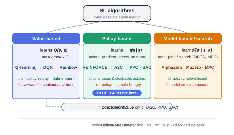
Plus one more axis: online (interact while learning) vs. offline (learn from a fixed logged dataset — often the realistic setting in science and medicine).
In this section#
- Value-based algorithms — Q-learning, DQN, Rainbow
- Policy-based algorithms — A2C, PPO, SAC
- Model-based algorithms - AlphaZero, MuZero, MPC
DQN: Q-learning with a network (2013–2015)#
Naively regressing on the TD target diverges: the data is sequentially correlated and the target moves with every update. DQN’s two fixes:
- Replay buffer — store transitions, train on random minibatches → breaks temporal correlation, reuses data.
- Target network — compute TD targets with a frozen copy $\theta^-$, updated only periodically → stabilizes the moving-target problem.
Result: one architecture, one hyperparameter set, superhuman on dozens of Atari games from raw pixels. More details in Value-based algorithms.
Policy gradients: optimize the policy directly#
Value-based methods struggle with continuous actions and stochastic policies. The alternative: parameterize $\pi_\theta$ and ascend the expected return $J(\theta) = \mathbb{E}_{\tau \sim \pi_\theta}[G(\tau)]$ directly. More details in Policy-based algorithms.
REINFORCE in one line of intuition:
$$ \nabla_\theta J(\theta) = \mathbb{E}_{\tau \sim \pi_\theta} \Big[ \sum_t \nabla_\theta \log \pi_\theta(a_t \mid s_t)\, G_t \Big] $$Increase the log-probability of actions in proportion to how much reward followed them.
For a DL audience: read this as “a loss function whose gradient points toward higher reward.” You already know everything after the gradient is computed — Adam, minibatches, the usual machinery.
Deep dive: the log-derivative trick (skipped live)
$\nabla_\theta \mathbb{E}_{x \sim p_\theta}[f(x)] = \mathbb{E}_{x \sim p_\theta}[f(x) \nabla_\theta \log p_\theta(x)]$, because $\nabla p_\theta = p_\theta \nabla \log p_\theta$. Applied to trajectories, the dynamics terms $P(s'|s,a)$ don’t depend on $\theta$, so only policy log-probs survive. This also explains the weakness: it’s a score-function estimator, hence high variance.
Actor-critic: taming the variance#
Subtract a learned baseline (the value function) to get the advantage $A(s,a) = Q(s,a) - V(s)$: “how much better was this action than average from here?” The actor ($\pi_\theta$) takes the gradient step; the critic ($V_\phi$) supplies the advantage estimate. (In practice: GAE for the advantage estimator.)
PPO: the workhorse#
Large policy updates from noisy advantage estimates cause collapse. PPO’s idea, in words: improve the policy, but don’t let any single update move it too far from the policy that collected the data. It does this by clipping the importance-sampling ratio $\rho_t = \pi_\theta(a_t|s_t) / \pi_{\theta_\text{old}}(a_t|s_t)$ into $[1-\epsilon,\, 1+\epsilon]$.
PPO is first-order, robust, and parallelizes well — which is why it became the default for robotics, games, and (as we’ll see next) RLHF.
The other branch: search + self-play#
AlphaGo → AlphaZero → MuZero combine learned value/policy networks with Monte Carlo tree search and self-play. Mentioned for the map, not covered today — but note AlphaTensor and AlphaDev applied exactly this recipe to algorithm discovery. More details in Model-based algorithms.