Q-table Worked Example: A 4×4 Gridworld#

One fully worked computation is worth ten abstractions. Consider a 4×4 grid: start in the top-left, a goal with reward $+1$ in the bottom-right, reward $0$ elsewhere, actions {up, down, left, right}, $\gamma = 0.9$.

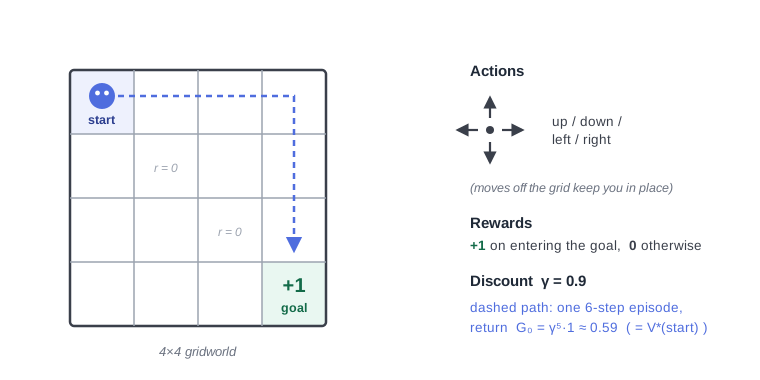
The dashed path shows one possible episode: 6 steps to the goal, so its return is $G_0 = \gamma^5 \cdot 1 \approx 0.59$ — the single $+1$ reward, discounted once per step of delay. Value iteration below will confirm this is in fact the optimal value of the start state.

Value iteration by hand (first two sweeps)#

Initialize $V_0(s) = 0$ everywhere. Apply the Bellman optimality backup $V_{k+1}(s) = \max_a [R(s,a) + \gamma V_k(s')]$:

• Sweep 1: only the cells adjacent to the goal get value: they can reach it in one step, so $V_1 = 1$ there (reward on entering the goal), $0$ elsewhere.
• Sweep 2: cells two steps away become $\gamma \cdot 1 = 0.9$; the adjacent cells stay $1$.
• Value “radiates” outward from the goal, discounted per step: $1,\ 0.9,\ 0.81,\ 0.729, \dots$

The greedy policy with respect to the converged $V^*$ simply walks downhill in distance-to-goal — as it should.

The same thing in code#

import numpy as np

N, gamma = 4, 0.9
V = np.zeros((N, N))
goal = (N - 1, N - 1)
moves = [(-1, 0), (1, 0), (0, -1), (0, 1)]

for sweep in range(50):
    V_new = np.zeros_like(V)
    for i in range(N):
        for j in range(N):
            if (i, j) == goal:
                continue
            best = -np.inf
            for di, dj in moves:
                ni = min(max(i + di, 0), N - 1)
                nj = min(max(j + dj, 0), N - 1)
                r = 1.0 if (ni, nj) == goal else 0.0
                best = max(best, r + gamma * V[ni, nj])
            V_new[i, j] = best
    V = V_new

print(np.round(V, 3))

Output — value radiating from the goal, $\gamma^{d-1}$ for a cell $d$ steps away:

[[0.59  0.656 0.729 0.81 ]     # start: 6 steps away ⇒ 0.9^5 ≈ 0.59
 [0.656 0.729 0.81  0.9  ]     # constant along anti-diagonals
 [0.729 0.81  0.9   1.   ]     # (equal distance to goal)
 [0.81  0.9   1.    0.   ]]    # goal itself: terminal, V = 0

Note two things worth pointing out: the start-state value $0.59$ matches the return of the 6-step episode in the figure above, and the goal cell stays $0$ — it is terminal, and the $+1$ is collected on entering it, not for being there.

Point of the demo: the entire solution came from repeatedly applying one local consistency rule. No gradient descent, no data set — just the Bellman operator. Deep RL replaces the table V[i, j] with a neural network; everything else is engineering around that substitution.