When Generative AI Is Guessing: Separating What a Model Knows from What It Makes Up

Generative AI can produce a thousand plausible-looking forecasts, scenarios, or synthetic records. The hard question is which ones to trust. In a paper accepted at AISTATS 2026, my coauthors and I give a precise answer to a narrower question that turns out to be the right one: for each output, how much of its variation comes from the model not knowing?

Generative models in the back office

Most public attention to generative AI goes to chatbots and image generators. The quieter growth is in generative models that produce numbers rather than words: synthetic demand curves for products that have not launched, simulated price paths for stress-testing a portfolio, artificial sensor traces for equipment that has not yet failed, privacy-preserving stand-ins for customer records that cannot leave a secure environment.

The workhorse for much of this is the diffusion model, the same family of methods behind the leading image generators. A diffusion model learns to produce new samples that look like its training data by starting from pure noise and removing the noise step by step, hundreds of times, until a plausible sample remains. Each run starts from different noise, so each run gives a different sample. That is the point. A planner wants a thousand different demand scenarios, not one.

But the randomness that makes these models useful also hides a problem. When one of the thousand scenarios looks strange, there are two possible explanations. The model may be exploring a real possibility that is simply unusual. Or the model may have wandered into territory it never learned, where it is producing confident-looking output with no basis. A planner needs to know which, and the model’s output alone does not say.

Two kinds of uncertainty

Statisticians have names for these two explanations.

Aleatoric uncertainty is the randomness built into the process. The word comes from the Latin for dice. If you flip a fair coin, there is no amount of additional study that will tell you how the next flip lands. In a diffusion model, the noise injected at each step is aleatoric: it is there by design, and more training data will not remove it.

Epistemic uncertainty is uncertainty about what the model has learned. The word comes from the Greek for knowledge. It arises because the model’s parameters were fit to finite data, and many different parameter settings would have fit that data about equally well. Where those settings agree, the model knows. Where they disagree, the model is guessing. Unlike aleatoric uncertainty, epistemic uncertainty shrinks with more data or a better model.

For anyone deciding whether to act on a generated output, the distinction is the whole game. Aleatoric variation is a feature. Epistemic variation is a warning.

The two can be separated formally. For one step of generation, the total variability of the next state decomposes by the law of total covariance into an average of the within-model randomness plus the variability of the model’s prediction across plausible parameter values. Writing the parameters as theta:

\[\operatorname{Cov}(x_{t-1} \mid x_t) \;=\; \underbrace{\mathbb{E}_{\theta}\big[\operatorname{Cov}(x_{t-1} \mid x_t, \theta)\big]}_{\text{aleatoric}} \;+\; \underbrace{\operatorname{Cov}_{\theta}\big[\mathbb{E}(x_{t-1} \mid x_t, \theta)\big]}_{\text{epistemic}}\]

The first term is what a fixed model would do on its own: injected noise. The second is how much the prediction moves when you perturb the parameters within the range the data cannot rule out. Our paper is about computing the second term, and only the second term, for a diffusion model.

That sounds simple. It is not, for two reasons: the second term depends on a distribution over parameters that no one can compute exactly for a modern neural network, and whatever we compute for one step has to be carried through hundreds of steps.

Why diffusion models make this hard

A diffusion model does not produce its output in one shot. It produces a trajectory. Starting from noise at step T, the network predicts how to denoise a little, the sampler applies that prediction plus a fresh dose of random noise, and the process repeats until step 0 yields the sample. A typical run has several hundred steps.

This matters for uncertainty because small modeling errors compound. If the network is slightly unsure at step 400, the state it hands to step 399 is slightly off, and step 399 was never trained on states that are slightly off in that way, so it is slightly more unsure, and so on. By step 0 the accumulated epistemic uncertainty can be large even if no single step was badly wrong. The regions where this happens are predictable in principle: between clusters of training data, at the edges of the training distribution, and anywhere the training set was thin.

The common practical shortcut is to measure total variance across samples and treat it as a proxy for reliability. But total variance is the whole left-hand side of the equation above, aleatoric and epistemic together. A sample can have high total variance because the process is supposed to be random there, and low total variance in a region the model never learned. The proxy does not distinguish the two cases, and in our experiments it misses exactly the samples one would most want to catch.

Isolating the epistemic part

Our method has three ingredients, each with a standard name.

The Laplace approximation. The ideal object is the posterior distribution over parameters: given the training data, which parameter settings are plausible and how plausible is each. For a neural network this distribution is intractable. The Laplace approximation replaces it with a Gaussian centered at the trained parameters, with a covariance that reflects how sharply the training loss curves around that point. Directions in which the loss rises steeply are directions the data has pinned down; directions in which it is flat are directions the data leaves open. Those flat directions are where epistemic uncertainty lives.

Fisher information. The curvature that defines that Gaussian is, for a model trained by squared error, the Fisher information matrix, a quantity that goes back to R. A. Fisher in the 1920s and measures how much the data tells you about each parameter. In a neural network it is approximated by averaging the outer products of the network’s gradients over the training set. Its inverse, lightly regularized, is the parameter covariance we need:

\[\Sigma_{\theta} \;\approx\; (H + \lambda I)^{-1}, \qquad H \;\approx\; \frac{1}{n}\sum_{i=1}^{n} J_i^{\top} J_i\]

Here J_i is the gradient of the network’s output with respect to its parameters on the i-th training example, and lambda is a small constant that keeps the inverse well defined.

Propagation through the trajectory. At each denoising step, we ask how much the network’s prediction would move if the parameters were perturbed within that covariance. The answer is governed by the Jacobian J_t, the sensitivity of the step-t prediction to the parameters. The epistemic covariance of the next state is then the parameter covariance pushed through that sensitivity, and the recursion carries it forward step by step:

\[\Sigma^{\mathrm{ep}}_{t-1} \;=\; a_t^{2}\,\Sigma^{\mathrm{ep}}_{t} \;+\; b_t^{2}\, J_t\, \Sigma_{\theta}\, J_t^{\top}\]

where a_t and b_t are the sampler’s own step coefficients. Throughout, we hold the injected noise fixed, so that the only thing varying is the parameters. This is what makes the quantity epistemic and nothing else. At the end, each generated sample receives a single score, the trace of its accumulated epistemic covariance. A low score means the plausible parameter settings all agree about this sample. A high score means they do not.

The recursion has one simplification: it drops a cross-covariance term between successive steps. We checked this on eighty trajectories and found it changes the score by less than three hundredths of a percent.

Why the usual shortcut fails

The Fisher information matrix for a modern network is enormous: one row and one column per parameter, so a network with ten million parameters has a matrix with a hundred trillion entries. Nobody computes it in full.

The standard workaround is the last-layer Laplace approximation, often abbreviated LLLA. It treats every layer of the network except the final one as fixed and known, and computes the Laplace approximation only over the final layer’s parameters. The final layer is small, so the matrix is tractable. This is the approach taken by BayesDiff, the most widely cited prior method for uncertainty in diffusion models, and by much of the broader literature on Bayesian deep learning.

The trouble is that the final layer is not where most of the uncertainty is. A neural network’s early and middle layers learn the features; the final layer only combines them. If the features themselves are unreliable in some region, because the training data was sparse there, the last layer cannot see that. It reports confidence in a combination of features that were never trustworthy to begin with.

A small example makes this concrete. Train a diffusion model on data that forms nine tight clusters arranged in a three-by-three grid. Then generate samples and score them. Some samples will land between clusters, in regions where there was no training data at all. Those are the samples a good uncertainty score should flag.

BayesDiff assigns low uncertainty to samples between the clusters. The last-layer approximation on its own suppresses the uncertainty even further. Our method assigns high epistemic uncertainty to exactly those between-cluster samples, and filtering by its score leaves samples clustered around the nine modes, as they should be. We also show that for a least-squares problem, the last-layer approximation carries no guarantee of recovering the true epistemic variance, while a random sample of parameters across all layers does.

Figure 1 from the paper. Top: uncertainty assigned to each generated sample by BayesDiff (left), last-layer Laplace (middle), and FLARE (right); blue is certain, brown is uncertain. Bottom: the samples that survive filtering at a fixed threshold.

In the paper’s figure, BayesDiff and the last-layer approximation assign low uncertainty to the samples between clusters, while FLARE assigns them high epistemic uncertainty and removes them on filtering.

A random slice is enough

If computing the full Fisher matrix is impossible and restricting to the last layer is wrong, what is left? Our answer is to pick parameters at random, from every layer of the network, and compute the Laplace approximation over that subset. We call the resulting estimator FLARE, for Fisher-Laplace Randomized Estimator.

The idea is that epistemic uncertainty is spread across the network, not concentrated in any one layer, so a uniformly random sample of parameters sees a representative share of it. Early layers contribute, middle layers contribute, and the final layer contributes in proportion to its actual importance rather than by fiat.

The question a statistician will ask is how large the sample must be. We prove that under standard conditions on the network’s gradient structure, the relative error of the FLARE estimate shrinks at the rate

\[\frac{\big|\operatorname{tr}(\widehat{\Sigma}^{\mathrm{ep}}) - \operatorname{tr}(\Sigma^{\mathrm{ep}})\big|}{\operatorname{tr}(\Sigma^{\mathrm{ep}})} \;=\; O\!\left(\frac{1}{\sqrt{m}}\right)\]

where m is the number of parameters sampled. The constants depend on how well conditioned the network’s gradients are and on how evenly information is spread across parameters, in a way the paper makes precise. The practical upshot is that the estimate improves predictably as the budget grows, and in our experiments it stabilizes once ten to thirty percent of parameters are included.

That rate is also what the last-layer approximation lacks. Fixing the subset to the final layer is a particular, non-random choice, and no analogous bound holds for it. The error of the last-layer estimate does not shrink as the layer gets bigger, because the layer was never the problem.

What we found

The practical use of an epistemic score is a filter. Generate many samples, score each, keep the fraction the model is most sure about, and discard the rest. No retraining, no ensembles of models, no repeated sampling.

We tested this on synthetic time series built to probe specific failure modes: sine waves with two competing frequencies, chirps whose frequency drifts over time, and damped oscillations. For each, we trained a diffusion model, generated samples, filtered them with each method, and measured how distinguishable the filtered samples were from real data. The measuring instrument is a separate classifier trained to tell real from generated. If it cannot do better than a coin flip, the generated samples are as good as real.

We report the result as gap closure: the fraction of the classifier’s advantage over chance that filtering removes. One hundred percent means the filtered samples are indistinguishable from real data. Zero means filtering did nothing. Negative means filtering made things worse.

On the sine benchmark, filtering with FLARE closed 93 percent of the gap. The last-layer approximation closed 47 percent. BayesDiff closed 13 percent. On chirps, the figures were 74, 59, and 42 percent. On damped sines, FLARE closed 85 percent, BayesDiff 10 percent, and the last-layer approximation came out at negative 19 percent: it kept the wrong samples.

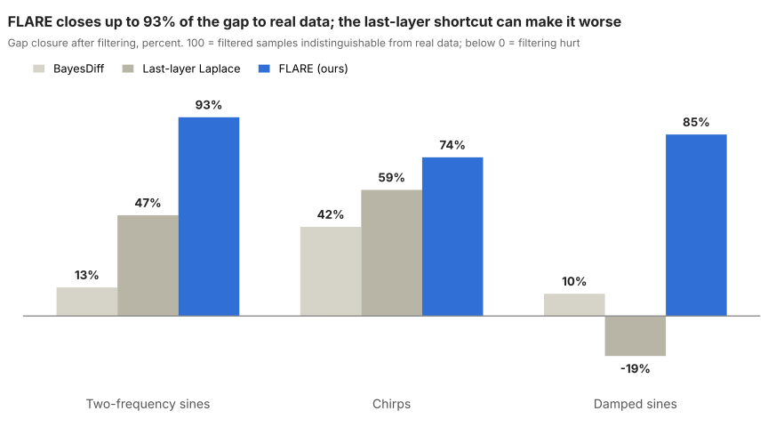
The bar below zero is the result to remember. On damped sines, the last-layer approximation ranked the samples backwards, so that keeping its most confident outputs produced a worse set than keeping none.

The filtered samples also look right. On the chirp task, FLARE removes the generated series with spurious oscillations and frequency drift, the kinds of artifacts a domain expert would reject on sight.

The evidence has limits, and the paper says so. The benchmarks are synthetic and low dimensional, chosen to isolate the phenomenon rather than to represent any industry. Extending to multivariate series and images is future work. Curvature estimation remains expensive for the largest models even with subsampling, and the natural next steps are structured sampling and low-rank approximations. None of the experiments use business data.

What this means

For practitioners who generate synthetic data to plan, stress-test, or train other systems, the result is a way to ask a generative model which of its outputs it would stand behind. The score is computed from the trained model as it stands. It requires no second model, no change to the generation process, and no human labeling. In a pipeline that produces thousands of scenarios, it is a cheap first pass that removes the ones the model had no business producing.

For researchers, the contribution is a clean separation that the field had been blurring. Total predictive variance in a diffusion model is not a measure of reliability, because it conflates designed randomness with ignorance. The epistemic term can be isolated, it can be propagated through a long sampling trajectory, and it can be estimated from a random fraction of the network with a convergence rate. The last-layer shortcut, which has become the default in Bayesian deep learning for reasons of cost, is shown to be the wrong default here, both empirically and in theory.

The broader point reaches beyond diffusion models. As generative systems move from producing text we can read to producing numbers we act on, the question of when the system is guessing becomes a question of risk management. It deserves the same precision we would demand of any other forecast.

About the paper

“Quantifying Epistemic Uncertainty in Diffusion Models,” by Aditi Gupta (Lawrence Berkeley National Laboratory and ICSI), Raphael A. Meyer (UC Berkeley and ICSI), Yotam Yaniv (Lawrence Berkeley National Laboratory), Elynn Chen (NYU Stern), and N. Benjamin Erichson (Lawrence Berkeley National Laboratory and ICSI). AISTATS 2026, the 29th International Conference on Artificial Intelligence and Statistics.

• Paper: arXiv:2602.09170

This work was supported in part by the U.S. Department of Energy, Office of Science, Office of Advanced Scientific Computing Research, and by DARPA.